Balbharati Maharashtra State Board11th Commerce Maths Solution Book PdfChapter 1 Partition Values Miscellaneous Exercise 1 Questions and Answers.
Maharashtra State Board 11th Commerce Maths Solutions Chapter 1 Partition Values Miscellaneous Exercise 1
Solution & Step-by-Step Answer:
The given data can be arranged in ascending order as follows: 1, 2, 2, 2, 2, 3, 3, 3, 3, 3, 4, 4, 4, 5, 6 Here, n = 15 Q2 = value of 2 observation = value of 2 observation = value of (2 × 4)th observation = value of 8th observation ∴ Q2 = 3 P17 = value of 17 observation = value of 17 observation = value of (17 × 0.16)th observation = value of (2.72)th observation = value of 2nd observation + 0.72 (value of 3rd observation – value of 2nd observation) = 2 + 0.72 (2 – 2) ∴ P17 = 2 D7 = value of 7 observation = value of 7 observation = value of (7 × 1.6)th observation = value of (11.2)th observation = value of 11th observation + 0.2(value of 12th observation – value of 11th observation) = 4 + 0. 2(4 – 4) ∴ D7 = 4
Solution & Step-by-Step Answer:
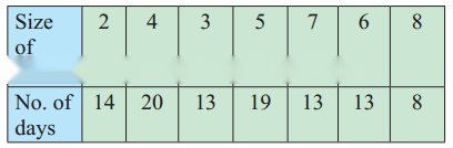
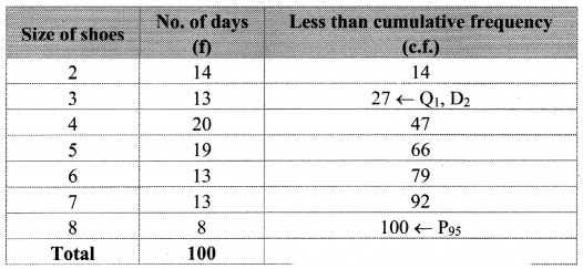
By arranging the given data in ascending order, we construct the less than cumulative frequency table as given below: Here, n = 100 Q1 = value of observation = value of observation = value of (25.25)th observation Cumulative frequency which is just greater than (or equal) to 25.25 is 27. ∴ Q1 = 3 D2 = value of 2 observation = value of 2 observation = value of (2 × 10.1)th observation = value of (20.2)th observation Cumulative frequency which is just greater than (or equal) to 20.2 is 27. ∴ D2 = 3 P95 = value of 95 observation = value of 95 observation = value of (95 × 1.01)th observation = value of (95.95)th observation The cumulative frequency which is just greater than (or equal) to 95.95 is 100. ∴ P95 = 8
Solution & Step-by-Step Answer:
Marks in Mathematics can be arranged in ascending order as follows: 23, 23, 25, 25, 32, 35, 36, 37, 38, 42 Here, n = 10 ∴ Median = value of observation Median = value of observation = value of (5.5)th observation = value of 5th observation + 0.5(value of 6th observation – value of 5th observation) = 32 + 0.5 (35 – 32) = 32 + 0.5(3) = 32 + 1.5 = 33.5 Marks in Statistics can be arranged in ascending order as follows: 22, 23, 26, 28, 29, 32, 34, 36, 45, 50 Here, n = 10 ∴ Median = value of observation = value of observation = value of (5.5)th observation = value of 5th observation + 0.5(value of 6th observation – value of 5th observation) = 29 + 0.5(32 – 29) = 29 + 0.5(3) = 29 + 1.5 = 30.5 ∴ Median marks for Mathematics = 33.5 and Median marks for Statistics = 30.5 ∴ The level of knowledge in Mathematics is higher than that of Statistics.

Solution & Step-by-Step Answer:
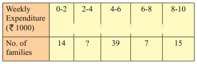
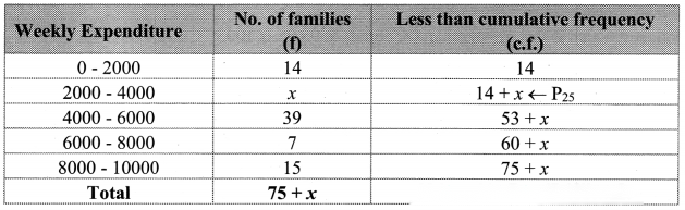
Let x be the missing frequency of expenditure group 2000 – 4000. We construct the less than cumulative frequency table as given below: Here, N = 75 + x Given, P25 = 2880 ∴ P25 lies in the class 2000 – 4000. ∴ L = 2000, h = 2000, f = x, c.f. = 14 ∴ P25 = L + ∴ 2880 = 2000 + ∴ 2880 – 2000 = ∴ 880x = 500(x + 19) ∴ 880x = 500x + 9500 ∴ 880x – 500x = 9500 ∴ 380x = 9500 ∴ x = 25 ∴ 25 is the missing frequency of the expenditure group 2000 – 4000.
Solution & Step-by-Step Answer:
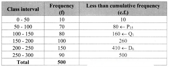
Since the difference between any two consecutive mid values is 50, the width of each class interval is 50. ∴ the class intervals will be 0 – 50, 50 – 100, etc. We construct the less than cumulative frequency table as given below: Here, N = 500 Q1 class = class containing observation ∴ = 125 Cumulative frequency which is just greater than (or equal) to 125 is 160. Q1 lies in the class 100 – 150. ∴ L = 100, h = 50, f = 80, c.f. = 80 ∴ Q1 = L + = 100 + (125 – 80) = 100 + (45) = 100 + 28.125 = 128.125 D6 class = class containing observation ∴ = 300 Cumulative frequency which is just greater than (or equal) to 300 is 410. ∴ D6 lies in the class 200 – 250. ∴ L = 200, h = 50, f = 150, c.f. = 260 ∴ D6 = L + = 200 + (300 – 260) = 200 + (40) = 200 + 13.33 = 213.33 P15 class = class containing observation ∴ = 75 Cumulative frequency which is just greater than (or equal) to 75 is 80. ∴ P15 lies in the class 50 – 100. ∴ L = 50, h = 50, f = 70, c.f. = 10 ∴ P15 = L + = 50 + (75 – 10) = 50 + (65) = 50 + = 50 + 46.4286 = 96.4286 ∴ Q1 = 128.125, D6 = 213.33, P15 = 96.4286

Solution & Step-by-Step Answer:
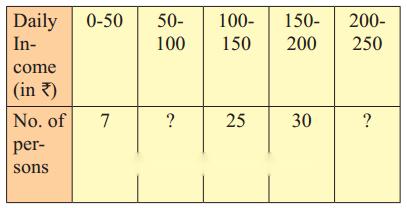
Let a and b be the missing frequencies of class 50 – 100 and class 200 – 250 respectively. We construct the less than cumulative frequency table as given below: Here, N = 62 + a + b Since, N = 100 ∴ 62 + a + b = 100 ∴ a + b = 38 ……(i) Given, P30 = 110 ∴ P30 lies in the class 100 – 150. ∴ L = 100, h = 50, f = 25, c.f. = 7 + a = 30 ∴ P30 = L + ∴ 110 = 100 + [30 – (7 + a)] ∴ 110 – 100 = 2(30 – 7 – a) ∴ 10 = 2(23 – a) ∴ 5 = 23 – a ∴ a = 23 – 5 ∴ a = 18 Substituting the value of a in equation (i), we get 18 + b = 38 ∴ b = 38 – 18 ∴ b = 20 ∴ 18 and 20 are the missing frequencies of the class 50 – 100 and class 200 – 250 respectively.

Solution & Step-by-Step Answer:
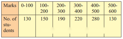
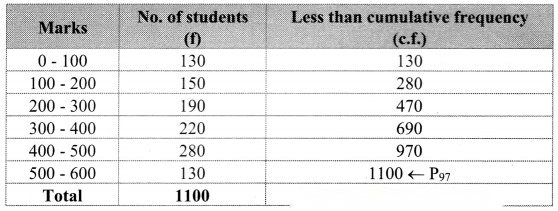
To decide cut-off marks for qualifying for an examination when 3% of students pass, we have to find P97. We construct the less than cumulative frequency table as given below: Here, N = 1100 P97 class = class containing observation ∴ = 1067 Cumulative frequency which is just greater than (or equal) to 1067 is 1100. ∴ P97 lies in the class 500 – 600. ∴ L = 500, h = 100, f = 130, c.f. = 970 ∴ P97 = L + = 500 + (1067 – 970) = 500 + (97) = 500 + 74.62 = 574.62 ~ 575 ∴ the cut off marks for qualifying an examination is 575.
Solution & Step-by-Step Answer:
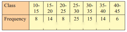
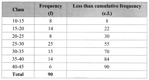
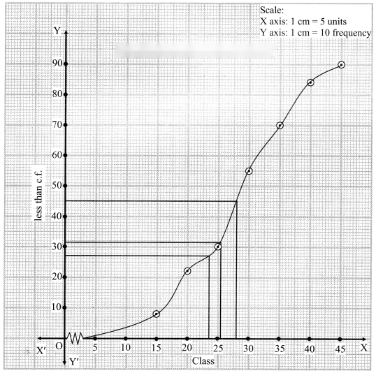
To draw an ogive curve, we construct the less than cumulative frequency table as given below: The points to be plotted for less than ogive are (15, 8), (20, 22), (25, 30), (30, 55), (35, 70), (40, 84), (45, 90). N = 90 For median, consider = 45 For D3, consider = 27 For P35, consider = 31.5 ∴ We take the values 45, 27 and 31.5 on the Y-axis and draw lines from these points parallel to X-axis. From the points where they intersect the less than ogive, we draw perpendicular on the X-axis. Foot of the perpendicular represent the values of median, D3 and P35 respectively. ∴ Median ~ 29, D3 ~ 23.5, P35 ~ 26
Solution & Step-by-Step Answer:
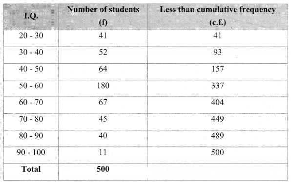
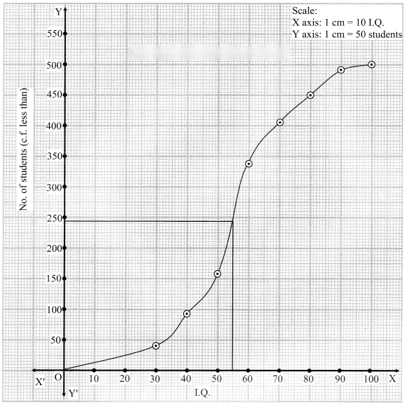
To draw an ogive curve, we construct the less than cumulative frequency table as given below: The points to be plotted for less than ogive are (30, 41), (40, 93), (50, 157), (60, 337), (70, 404), (80, 449), (90, 489), (100, 500) To find the number of students whose I.Q. is more than 55, we consider the value 55 on the X-axis. From this point, we draw a line that is parallel to Y-axis. From the point this line intersects the less than ogive, we draw a perpendicular on the Y-axis. The foot of perpendicular gives the number of students whose I.Q. is less than 55. ∴ The foot of perpendicular ~ 244 ∴ No. of students whose I.Q. is less than 55 ~ 244 ∴ No. of Students whose I.Q. is more than 55 = 500 – 244 = 256

Solution & Step-by-Step Answer:
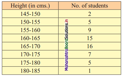
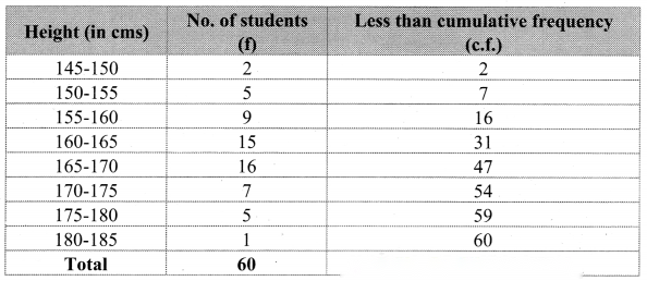
To draw an ogive curve, we construct the less than cumulative frequency table as given below: The points to be plotted for less than ogive are (150, 2), (155, 7), (160, 16), (165, 31), (170, 47), (175, 54), (180, 59) and (185, 60). N = 60 ∴ = 30 ∴ We take the value 30 on the Y-axis and from this point, we draw a line parallel to X-axis. From the point where this line intersects the less than ogive, we draw a perpendicular on X-axis. The foot perpendicular gives the value of the median. ∴ Median ~ 164.67 Now, let us calculate the median from the mathematical formula. ∴ = 30 The median lies in the class interval 160 – 165. ∴ L = 160, h = 5, f = 15, c.f. = 16 Median = L + = 160 + (30 – 16) = 160+ × 14 = 160 + 4.67 = 164.67

Solution & Step-by-Step Answer:
n = 25 Median = = 13th observation We have been stated that 7 students failed (assuming passing marks on 35) and 6 students got distinction (assuming distinction as 70+), and the marks of the remaining 12 students (who will be situated between the two groups mentioned above, if arranged in ascending order), we have, F, F, F, F, F, F, F, 36, 37, 38, 39, 41, 41, 44, 52, 56, 59, 61, 64, D, D, D, D, D, D ∴ median = 13th observation = 41.
Solution & Step-by-Step Answer:
n = 79 Median = 55kg Lowest observation = 53 kg Flighest observation = 59 kg 6 new students are added to the group having weights in Kg as follows: 50, 51, 52, 59.5, 60, 61 From the above, we see that of the 6 new students, 3 have weights which are below the lowest weight of the earlier group and 3 have weights which are above the highest weight of the earlier group. ∴ the median remains the same ∴ median = 55 kg.
Solution & Step-by-Step Answer:
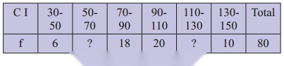
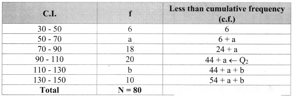
Let a and b be the missing frequencies of class 50 – 70 and class 110 – 130 respectively. We construct the less than cumulative frequency table as given below: Here, N = 54 + a + b Since, N = 80 ∴ 54 + a + b = 80 ∴ a + b = 26 …..(i) Given, Median = Q2 = 92 ∴ Q2 lies in the class 90 – 110. ∴ L = 90, h = 20, f = 20, c.f. = 24 + a = 40 ∴ Q2 = L + ∴ 92 = 90 + [40 – (24 + a) ∴ 92 – 90 = 40 – 24 – a ∴ 2 = 16 – a ∴ a = 14 Substituting the value of a in equation (i), we get 14 + b = 26 ∴ b = 26 – 14 = 12 ∴ 14 and 12 are the missing frequencies of the class 50 – 70 and class 110 – 130 respectively.
Solution & Step-by-Step Answer:
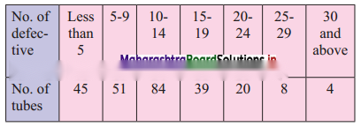
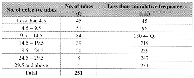
To find the number of defective tubes in the central batch, we have to find Q2. Since the given data is not continuous, we have to convert it into a continuous form by subtracting 0.5 from the lower limit and adding 0.5 to the upper limit of every class interval. ∴ the class intervals will be Less than 4.5, 4.5 – 9.5, etc. We construct the less than cumulative frequency table as given below: Here, N = 251 Q2 class = class containing observation ∴ = 125.5 Cumulative frequency which is just greater than (or equal to) 125.5 is 180. ∴ Q2 lies in the class 9.5 – 14.5. ∴ L = 9.5, h = 5, f = 84, c.f. = 96 ∴ Q2 = L + = 9.5 + (125.5 – 96) = 9.5 + × 29.5 = 9.5 + = 9.5 + 1.76 = 11.26
Solution & Step-by-Step Answer:
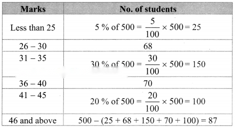
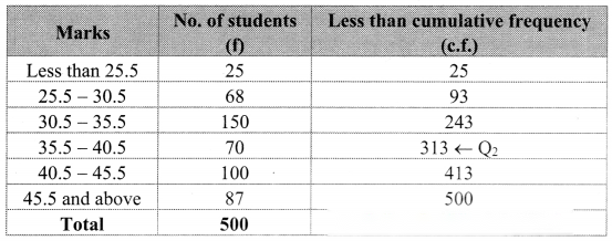
Given data can be written in tabulated form as follows: Since the given data is not continuous, we have to convert it into the continuous form by subtracting 0.5 from the lower limit and adding 0.5 to the upper limit of every class interval. ∴ the class intervals will be Less than 25.5, 25.5 – 30.5, etc. We construct the less than cumulative frequency table as given below: Here, N = 500 Q2 class = class containing observation ∴ = 250 Cumulative frequency which is just greater than (or equal to) 250 is 313. ∴ Q2 lies in the class 35.5 – 40.5. ∴ L = 35.5, h = 5, f = 70, c.f. = 243 ∴ Median = Q2 = L + = 35.5 + (250 – 243) = 35.5 + (7) = 35.5 + 0.5 = 36
Solution & Step-by-Step Answer:
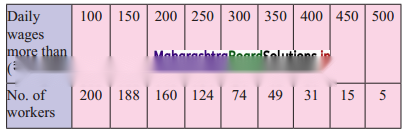
For more than ogive points to be plotted are (100, 200), (150, 188), (200, 160), (250, 124), (300, 74), (350, 49), (400, 31), (450, 15), (500, 5) Here, N = 200 For Q1, = 4 For Q3, = 150 We take the points having Y co-ordinates 50 and 150 on Y-axis. From these points, we draw lines which are parallel to X-axis. From the points of intersection of these lines with the curve, we draw perpendicular on X-axis. X-Co-ordinates of these points gives the values of Q1 and Q3. Since X-axis has daily wages more than and not less than the given amounts. ∴ Q1 = Q3 and Q3 = Q1 ∴ Q2 ~ 215, Q3 ~ 348
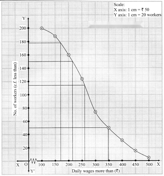
(i) To find the number of workers with daily wages between ₹ 170 and ₹ 260,
Take the values 170 and 260 on X-axis. From these points, we draw lines parallel to Y-axis.
From the point where they intersect the more than ogive, we draw perpendiculars on Y-axis.
The points where they intersect the Y-axis gives the values 178 and 114.
∴ Number of workers having daily wages between ₹ 170 and ₹ 260 = 178 – 114 = 64
(ii) To find the number of workers having daily wages less than ₹ 260, we consider the value 260 on the X-axis.
From this point, we draw a line that is parallel to Y-axis.
From the point where the line intersects the more than ogive, we draw a perpendicular on the Y-axis.
The foot of perpendicular gives the number of workers having daily wages of more than 260.
The foot of perpendicular ~ 114
∴ No. of workers whose daily wages are more than ₹ 260 ~ 114
∴ No. of workers whose daily wages are less than ₹ 260 = 200 – 114 = 86
Solution & Step-by-Step Answer:
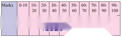
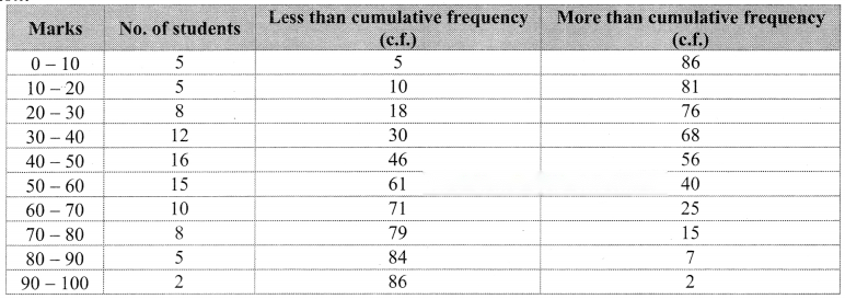
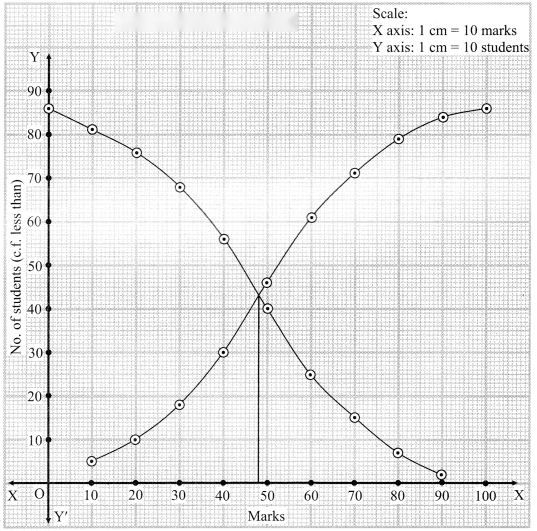
For less than given points to be plotted are (10, 5), (20, 10), (30, 18), (40, 30), (50, 46), (60, 61), (70, 71), (80, 79), (90, 84), (100, 86) For more than given points to be plotted are (0, 86), (10, 81), (20, 76), (30, 68), (40, 56), (50, 40), (60, 25), (70, 15), (80, 7), (90, 2) From the point of intersection of two ogives. We draw a perpendicular on X-axis. The point where it meets the X-axis gives the value of the median.
Solution & Step-by-Step Answer:
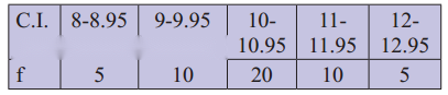
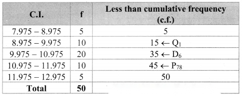
Since the given data is not in the form of a continuous frequency distribution, we have to convert it into that form by subtracting 0.025 from the lower limit and adding 0.025 to the upper limit of each class interval. ∴ the class intervals will be 7.975 – 8.975, 8.975 – 9.975, etc. We construct the less than cumulative frequency table as given below: Here, N = 50 Q1 class = class containing observation ∴ = 12.5 Cumulative frequency which is just greater than (or equal) to 12.5 is 15. ∴ Q1 lies in the class 8.975 – 9.975. ∴ L = 8.975, h = 1, f = 10, c.f. = 5 Q1 = L + = 8.975 + (12.5 – 5) = 8.975 + 0.1(7.5) = 8.975 + 0.75 = 9.725 D6 class = class containing observation ∴ = 30 Cumulative frequency which is just greater than (or equal) to 30 is 35. ∴ D6 lies in the class 9.975 – 10.975. ∴ L = 9.975, h = 1, f = 20, c.f. = 15 D6 = L + = 9.975 + (30 – 15) = 9.975 + 0.05(15) = 9.975 + 0.75 = 10.725 P78 class = class containing observation = 39 Cumulative frequency which is just greater than (or equal) to 39 is 45. ∴ P78 lies in the class 10.975 – 11.975. ∴ L = 10.975, h = 1, f = 10, c.f. = 35 ∴ P78 = L + = 10.975 + (39 – 35) = 10.975 + 0.1(4) = 10.975 + 0.4 = 11.375
Solution & Step-by-Step Answer:
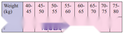
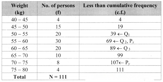
We construct the less than cumulative frequency table as given below: Here, N = 111 Q1 class = class containing observation ∴ = 27.75 Cumulative frequency which is just greater than (or equal) to 27.75 is 39. ∴ Q1 lies in the class 50 – 55. ∴ Q1 = L + = 50 + (27.75 – 19) = 50 + × 8.75 = 50 + 2.1875 = 52.1875 Q2 class = class containing observation ∴ = 55.5 Cumulative frequency which is just greater than (or equal) to 55.5 is 69. ∴ Q2 lies in the class 55 – 60. ∴ L = 55, h = 5, f = 30, c.f. = 39 ∴ Q2 = L + = 55 + (55.5 – 39) = 55 + × 16.5 = 55 + 2.75 = 57.75 Q3 class = class containing observation ∴ = 83.25 Cumulative frequency which is just greater than (or equal) to 83.25 is 89. ∴ Q3 lies in the class 60 – 65. ∴ L = 60, h = 5, f = 20, c.f. = 69 ∴ Q3 = L + = 60 + (83.25 – 69) = 60 + × 14.25 = 60 + 3.5625 = 63.5625 In order to find the number of persons between 57 kg and 72 kg, We need to find x in Px, where Px = 57 kg and y in Py, where Py = 72 kg Then (y – x) would be the % of persons weighing between 57 kg and 72 kg Px = 57 ∴ L + = 57 ∴ 55 + (1.11x – 39) = 57 ∴ (1.11x – 39) = 2 ∴ 1.11x – 39 = 12 ∴ 1.11x = 51 ∴ x = 45.95 ∴ Py = 72 ∴ L + = 72 ∴ 70 + (1.11y – 99) = 72 ∴ 0.625(1.11y – 99) = 2 ∴ 1.11y – 99 = 3.2 ∴ 1.11y = 102.2 ∴ y = 92.07 ∴ % of people weighing between 57 kg and 72 kg = 92.07 – 45.95 = 46.12 % ∴ No. of people weighing between 57 kg and 72 kg = 111 × 46.12% = 51.1932 ~ 51
Solution & Step-by-Step Answer:
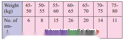
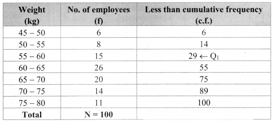
We construct the less than cumulative frequency table as given below: Here, N = 100 Q1 class = class containing observation ∴ = 25 Cumulative frequency which is just greater than (or equal) to 25 is 29. ∴ Q1 lies in the class 55 – 60. ∴ L = 55, h = 5, f = 15, c.f. = 14 ∴ Q1 = L + = 55 + (25 – 14) = 55 + × 11 = 55 + 3.67 = 58.67 ∴ Maximum weight of the lightest 25% of employees is 58.67 kg.